Learning with Amplitude Amplification
This blog series aims at achieving two goals. Firstly, I want to learn more about the programming language Julia. Secondly, I want to experiment how Amplitude Amplification can be used as a learning algorithm despite its known limitiations. So in this blog entry, I will start to experiment a little and let’s see where I end up :)
Simple learning example with Amplitude Amplification Link to heading
In this initial exploration, let’s consider the simple case where we want to learn the Bernoulli distribution from examples. The Bernoulli distribution is characterized by the parameter $p \in [0,1]$ which is the probability to observe the value $1$ ( and $0$ is observed with probability $1-p$). Our goal here is to learn the parameter $p$ given $m$ samples from the Bernoulli distribution using the Amplitude Amplification routine. Let’s assume that $p=\frac{1}{4}$ and we are given the observations $0,1,0,0$, We then construct the following quantum circuit:
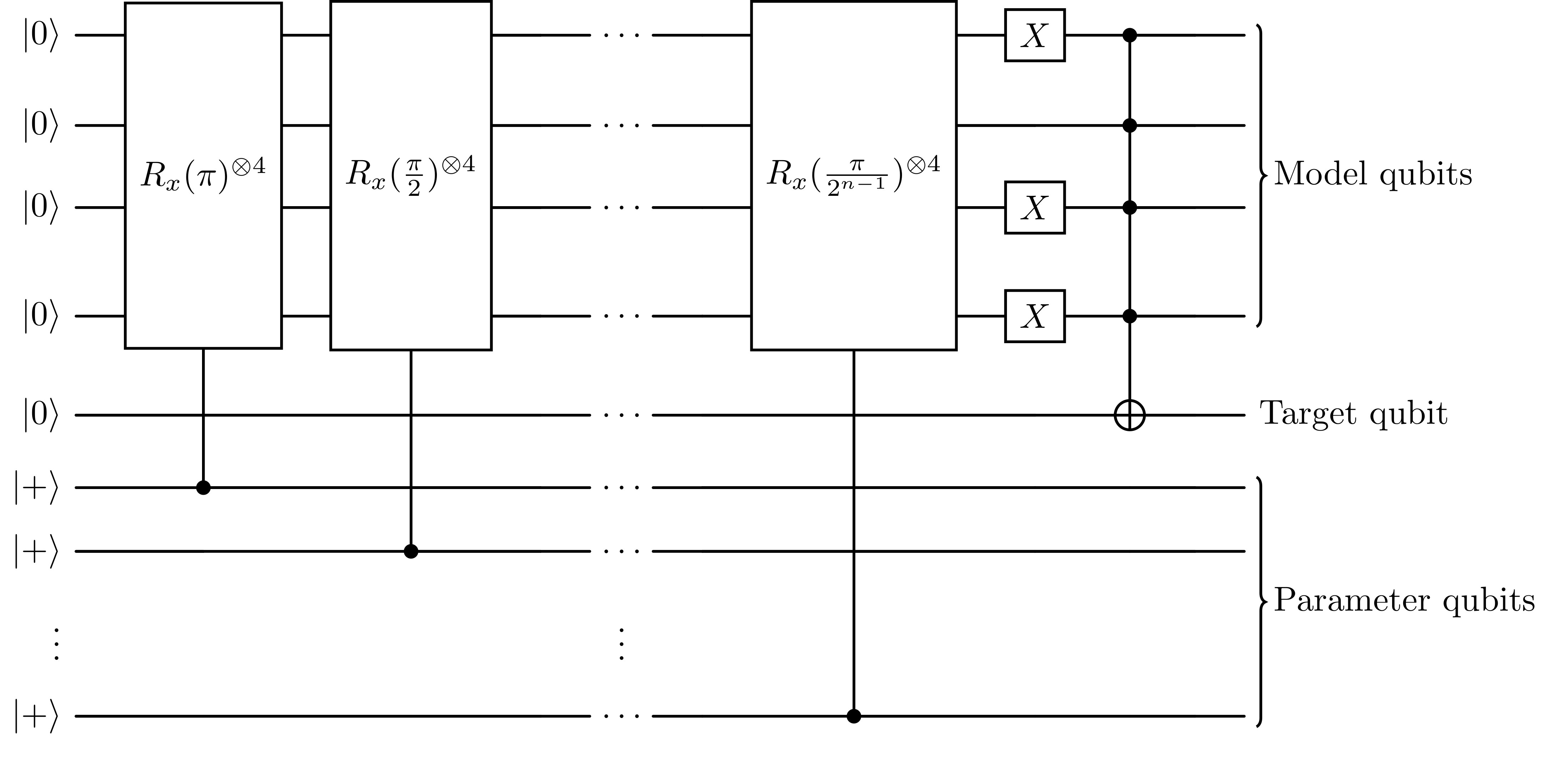
In this circuit we introduce 4 model qubits, where each qubit models the generation of one sample. As you can see, we model the Bernoulli distribution as a single qubit that is simply rotated around the X axis. We want to achieve that the models correctly represent the true distribution, which we do by introducing the target qubit. Additionally, we introduce parameter qubits, initially in the $|+\rangle^4$ state, where the amplitude of the correct parameter configuration is to be amplified. Intuitively, we want to find the most likely parameter configuration that generates the examples. We do this by amplifying those amplitudes, that correspond to the most likely parameter configuration. It is important to note that the AA subroutine only goes over the target and parameter qubits and NOT over the model qubits. This effectively allows us to use up to 40 or so parameter qubits realistically, before the runtime of AA explodes irresponsively, when usinig a fault-tolerant quantum computer. For classical simulations, we are bounded to about 20-30 parameter qubits or so (depending on if you have access to a super-computer).
After AA, measuring the parameter qubits then yields a quantum circuit model for the Bernoulli distribution, which we aim to learn. Additionally the parameter $p$ can be calculated.
The proof that AA indeed recovers $p$ can be found in the end of this section.
I think this method of modeling the distribution as a quantum circuit and then using AA to amplify the parameters that most likely generated the sample is quite simple, but might be useful. In the next section we will treat a little more complex distribution and showcase a “learning with AA” framework written in Julia.
Proof
Assuming the parameter register is in the state $\left|p_1\dots p_n\right>$, then the state before the multi-controlled CNOT in the end is given by: $$ \left | \psi_1 \right > = \bigotimes_{i=1}^{m} \left [ \cos( \sum_{j=1}^{n} \frac{p_j \pi}{2^{j-1}} )\left| \overline{y_i} \right> - i \sin( \sum_{j=1}^{n} \frac{p_j \pi}{2^{j-1}} ) \left| y_i \right> \right ] \otimes \left|0\right> \otimes \left|p_1\dots p_n\right> \ $$
Then after the multi-controlled CNOT, the part of the state that sets the target qubit to $1$ looks like: $$ \left | \psi_2 \right > = \prod_{i=1}^{m} \left [{1}(\overline{y_i}) \cos( \sum_{j=1}^{n} \frac{p_j \pi}{2^{j-1}} ) - {1}(y_i) i \sin( \sum_{j=1}^{n} \frac{p_j \pi}{2^{j-1}} ) \right ] \otimes \left| 1\dots 1 \right> \otimes \left|1\right> \otimes \left|p_1\dots p_n\right> + \dots\ $$ In amplitude amplification, we will find a configuration of the parameter qubits $\left| p_1,\dots,p_n \right>$, sucht that the amplitude of $\left| 1 \dots 1 \right>\left| 1 \right>$ in the model and target qubits is maximized. Thus the following quantity is maximized: $$ \prod_{i=1}^{m} \left [{1}(\overline{y_i}) \cos( \sum_{j=1}^{n} \frac{p_j \pi}{2^{j-1}} ) - {1}(y_i) i \sin( \sum_{j=1}^{n} \frac{p_j \pi}{2^{j-1}} ) \right ]^2 $$ Let us define $p:= \sum_{j=1}^{n} \frac{p_j \pi}{2^{j-1}} $, then straight forward calculation reveals that we maximize the following quantity: $$ [1-\sin^2(p)]^{\sum_i \overline{y_i}} \cdot [\sin^2(p)]^{\sum_i y_i}. $$ Computing the roots of the derivative with respect to $\sin^2(p)$ then reveals that the quantity above is maximized when $\sin^2(p) = \frac{\sum_i y_i}{m}$. And thus when we measure $p$ after running amplification amplification, we can simply compute $\sin^2(p)$ and have learned the parameters of the Bernoulli distribution.
More complex distributions Link to heading
To learn more complex distributions we will use a neat little project by a student of mine, which I supervised. The code of the project can be found here on github. This “learning with AA” framework let’s one even extend our circuits such that we can optimize not only over single qubit rotations, but also over arbitrary multi-qubit unitaries.
We will show a simple example of learning a quantum circuit using this AA learning framework.
The target distribution Link to heading
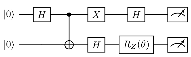
This is the circuit that generates the target distribution.
The model Link to heading
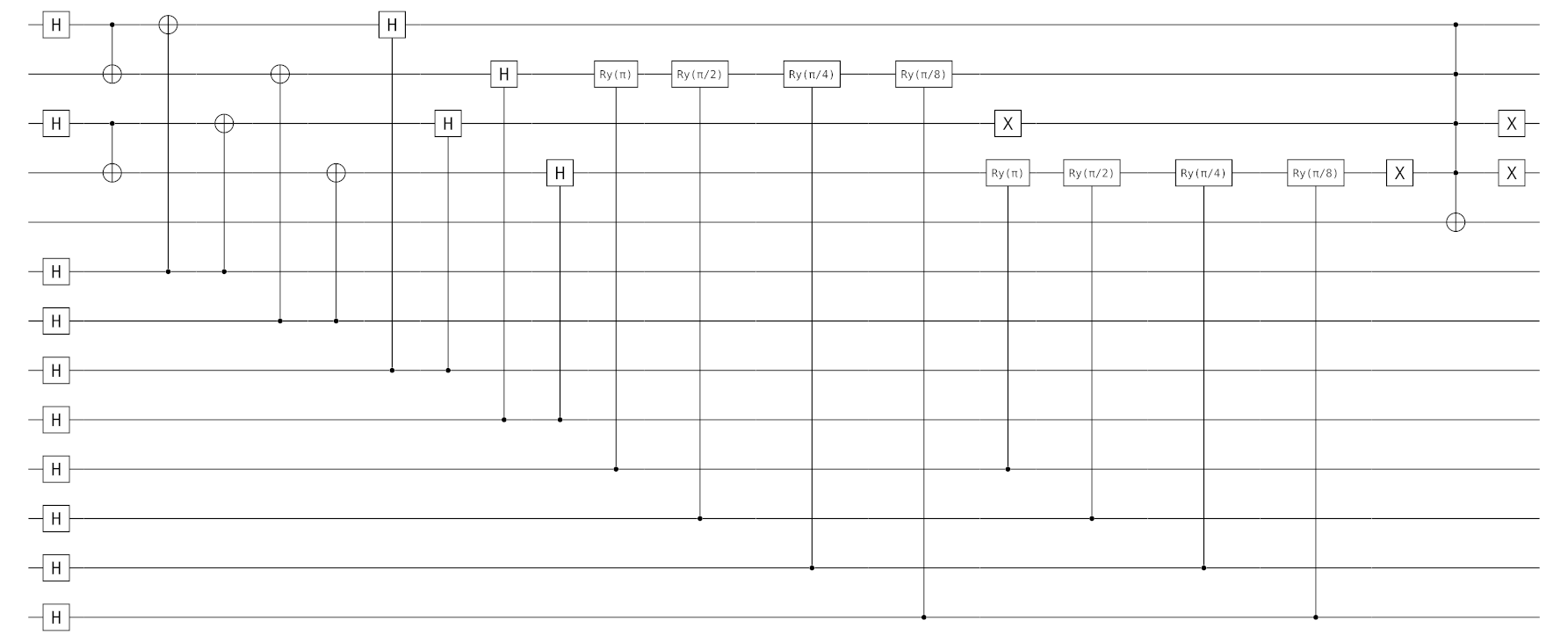
Here is the model we put forward in the complex distribution learning case: In this case the batch is [(1,1), (0,0)]
Simple learning example with Oblivious Amplitude Amplification Link to heading
One caveat of AA is that the input state to AA needs to be known. This really limits how we can use AA. For example it is not possible to use AA iteratively on different parts of a circuit. However there is Oblivious Amplitude Amplification, which lets one do AA when the input state is unknown. In this section I want to explore OAA a little bit and understand it better.
This, however, only works when the probability to observe the oracle qubit as, say, 1 is constant. Here we go a little bit on a tangent and explore Oblivious Amplitude Amplification (OAA). In OAA we are able to run AA on unknown input states, which normally is not possible. For reference, see these lecture notes here for an excellent explanation of Oblivious Amplitude Amplification. We will make heavy use of these lecture notes to derive our learning algorithm.
Learning an unkown qubit state Link to heading
The learning example we consider will actually not be a learning example in the sense that we don’t have any data. What we explore here is a very simple example of learning an unkown qubit state $|\phi\rangle$ using OAA.
As can be taken from the lecture notes, we require the “purified setting with indepedent initial weight”. This basically means we need the following conditions to be fulfilled:
- We have the promise that the state $\left| \psi \right>$ is composed of $l$ ancilla qubits followed by the ‘real’ state $|\phi\rangle$: that is, $\left| \psi \right>= \left| 0^l \right>\left| \phi \right>$
- We also have that $p(\psi) = p$ is independent of $\psi$, where $p(\psi) = \sum_{x:f(x)=1} |\alpha_x|^2$ is the probability to observe a good outcome.
Our strategy will be to have as input the unkown qubit state $\phi$ and then introduce an ancilla register. This already gives us condition 1. We then perform conditional rotations on the input state around the X/Y axes, conditioned on the ancilla register. Those conditional rotations are controlled by the ancilla register, right after putting the ancilla qubits in uniform superposition. This is done in such that the input state after the rotations will have a probability of $\frac{1}{2}$ to be measured as in the $|1\rangle$ basis state. This essentially gives us condition 2 above. The fact that the conditional rotations fulfill condition 2 is depicted in the following figure:
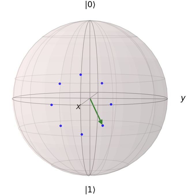
In the figure we can see, that any state that is put into a superposition over equi-distant rotations around the X axis, results in a state, that yields $|0\rangle$ or $|1\rangle$ with probability $\frac{1}{2}$.
Now, since we know that $p(\psi) = 0.5$, we only need a single round of OAA. In that case, we can do a neat trick I learned during this exploration: After entangling the input qubit with the ancilla register, we measure it. This results in 50/50 chance to observe 0/1. We want to measure 0. If we measure 1, we can force it back to 0 by using a sequence of rotations. The following figure depicts those rotations and their actions on the state in the two-domain view (see the lecture notes for full comprehension).
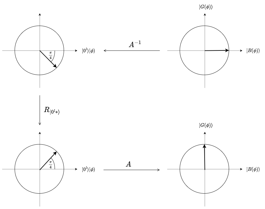
Now this all allows us to do two AA routines in sequence, which normally is not possible, since after the first, we don’t know the input state to the second. In this example of OAA, we will first learn a X rotation and then do AA to learn a Y rotation. The following Julia code does exactly what we described above. Let’s go through it step by step.
Let’s import Yao.jl as our quantum computing library and create some qubit state, that is unkown to us.
using Yao, YaoPlots

Φ = zero_state(1) |> Rx(-π/4) |> Ry(-π/4)
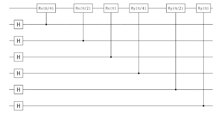
Now define our model architecture and the rotation around the clean ancillas.
# Define the parameterized rotations
# All of those need focus on 1st qb and 3 param qbs
RxChain = chain(4,repeat(H, 2:4),
            control(2, 1=>Rx(π/4)),
            control(3, 1=>Rx(π/2)),
            control(4, 1=>Rx(π)),
        );
RyChain = chain(4,repeat(H, 2:4),
            control(2, 1=>Ry(π/4)),
            control(3, 1=>Ry(π/2)),
            control(4, 1=>Ry(π)),
        );

model_architeture = chain(7, subroutine(RxChain, 1:4),
                            subroutine(RyChain, [1,5,6,7]))

YaoPlots.plot(model_architeture)

# Flip sign of all states that don't have clean ancillas
# This requires focus on the first and parameter qubits
R0lstar = chain(4, repeat(X, 2:4),
                    cz(2:3, 4),
                    repeat(X, 2:4)
                );
The first qubit is used to model the unkown qubit state. In our circuit we will input the unkown qubit state to the first qubit in the circuit above and search (AA) for the parameter configuration that tunes the qubit to 0. Measuring the parameter qubits allows us to then reconstruct parts of the unkown qubit state.
Now let’s run the actual algorithm:
# Add 6 zeros qubits for parameters
append_qubits!(Φ, 6);

# First parameterized rotation: Rx
focus!(Φ, 1:4)
Φ |> RxChain;
# Measure first qubit. For State tomography we want to force it to be 0.
outcome = measure!(Φ, 1)
if (outcome != 0)
    Φ |> Daggered(RxChain);
    Φ |> R0lstar;
    Φ |> RxChain;
end
relax!(Φ, 1:4)

# Second parameterized rotation: Ry
focus!(Φ, [1,5,6,7])
Φ |> RyChain;
# Measure first qubit. For State tomography we want to force it to be 0.
outcome = measure!(Φ, 1)
if (outcome != 0)
    Φ |> Daggered(RyChain);
    Φ |> R0lstar;
    Φ |> RyChain;
end
relax!(Φ, [1,5,6,7])
In the following plots we depict the distribution of the measurement probabilities for the parameter qubits:
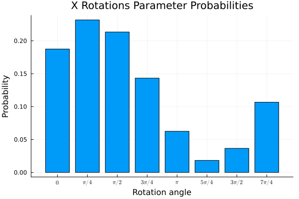
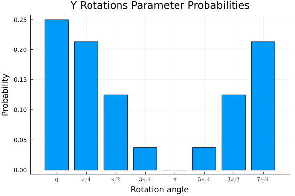
As we can see the amplitudes of the optimal configuration of the parameter qubits are amplified. Measuring the parameter qubits would then (with high probability) lead to a model for the input state.
Future work and open questions Link to heading
- Performance analysis? So far we went straight into the nitty-gritty without caring about performance.
- Can we “spike” the parameter distribution further? There is this paper which we might be able to use.
- Can we find some learning setting where the circuit model architecture is more complex and where we can use OAA iteratively for learning in a meaningful way?